


The following is Patrick Frank’s controversial article challenging data and climate models on global warming. Patrick Frank is a Ph.D. chemist with more than 50 peer-reviewed articles. He has previously published in Skeptic on the noble savage myth, as well as in Theology and Science on the designer universe myth and in Free Inquiry, with Thomas H. Ray, on the science is philosophy myth.
BUY this issue >
DOWNLOAD this article in PDF >
The claim that anthropogenic CO2 is responsible for the current warming of Earth climate is scientifically insupportable because climate models are unreliable
“He who refuses to do arithmetic is doomed to talk nonsense.”
“The latest scientific data confirm that the earth’s climate is rapidly changing. … The cause? A thickening layer of carbon dioxide pollution, mostly from power plants and automobiles, that traps heat in the atmosphere. … [A]verage U.S. temperatures could rise another 3 to 9 degrees by the end of the century … Sea levels will rise, [and h]eat waves will be more frequent and more intense. Droughts and wildfires will occur more often. Disease-carrying mosquitoes will expand their range. And species will be pushed to extinction.”
So says the National Resources Defense Council,2 with agreement by the Sierra Club,3 Greenpeace,4 National Geographic,5 the US National Academy of Sciences,6 and the US Congressional House leadership.7 Concurrent views are widespread,8 as a visit to the internet or any good bookstore will verify.
Since at least the 1995 Second Assessment Report, the UN Intergovernmental Panel on Climate Change (IPCC) has been making increasingly assured statements that human-produced carbon dioxide (CO2) is influencing the climate, and is the chief cause of the global warming trend in evidence since about 1900. The current level of atmospheric CO2 is about 390 parts per million by volume (ppmv), or 0.039% by volume of the atmosphere, and in 1900 was about 295 ppmv. If the 20th century trend continues unabated, by about 2050, atmospheric CO2 will have doubled to about 600 ppmv. This is the basis for the usual “doubled CO2” scenario.
Doubled CO2 is a bench-mark for climate scientists in evaluating greenhouse warming. Earth receives about 342 watts per square meter (W/m2) of incoming solar energy, and all of this energy eventually finds its way back out into space. However, CO2 and other greenhouse gases, most notably water vapor, absorb some of the outgoing energy and warm the atmosphere. This is the greenhouse effect. Without it Earth’s average surface temperature would be a frigid -19°C (-2.2 F). With it, the surface warms to about +14°C (57 F) overall, making Earth habitable.9
With more CO2, more outgoing radiant energy is absorbed, changing the thermal dynamics of the atmosphere. All the extra greenhouse gases that have entered the atmosphere since 1900, including CO2, equate to an extra 2.7 W/m2 of energy absorption by the atmosphere.10 This is the worrisome greenhouse effect.
On February 2, 2007, the IPCC released the Working Group I (WGI) “Summary for Policymakers” (SPM) report on Earth climate,11 which is an executive summary of the science supporting the predictions quoted above. The full “Fourth Assessment Report” (4AR) came out in sections during 2007.
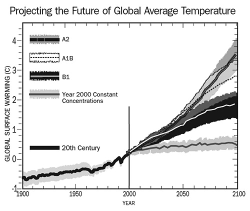
Figure 1. Projected increases in 21st century global average temperature assuming different CO2 emissions futures (described below). These projections are from the 4AR Special Report on Emissions Scenarios (SRES), and appear in Figure SPM-5 of the Working Group I “Summary for Policymakers”.11 The zero level was set to the average temperature between 1980–1999, which is why most of the 20th century shows negative values.
Figure 1 shows a black-and-white version of the “Special Report on Emission Scenarios” (SRES) Figure SPM-5 of the IPCC WGI, which projects the future of global average temperatures. These projections12 were made using General Circulation Models (GCMs). GCMs are computer programs that calculate the physical manifestations of climate, including how Earth systems such as the world oceans, the polar ice caps, and the atmosphere dynamically respond to various forcings. Forcings and feedbacks are the elements that inject or mediate energy flux in the climate system, and include sunlight, ocean currents, storms and clouds, the albedo (the reflectivity of Earth), and the greenhouse gases water vapor, CO2, methane, nitrous oxide, and chlorofluorocarbons.
In Figure 1, the B1 scenario assumes that atmospheric CO2 will level off at 600 ppmv, A1B assumes growth to 850 ppmv, and A2 reaches its maximum at a pessimistic 1250 ppmv. The “Year 2000” scenario optimistically reflects CO2 stabilized at 390 ppmv.
The original caption to Figure SPM-5 said, in part: “Solid lines are multi-model global averages of surface warming (relative to 1980–99) for the scenarios A2, A1B and B1, shown as continuations of the 20th century simulations. Shading denotes the plus/minus one standard deviation range of individual model annual averages.”
Well and good. We look at the projections and see that the error bars don’t make much difference. No matter what, global temperatures are predicted to increase significantly during the 21st century. A little cloud of despair impinges with the realization that there is no way at all that atmospheric CO2 will be stabilized at its present level. The Year 2000 scenario is there only for contrast. The science is in order here, and we can look forward to a 21st century of human-made climate warming, with all its attendant dangers. Are you feeling guilty yet?
But maybe things aren’t so cut-and-dried. In 2001, a paper published in the journal Climate Research13 candidly discussed uncertainties in the physics that informs the GCMs. This paper was very controversial and incited a debate.14 But for all that was controverted, the basic physical uncertainties were not disputed. It turns out that uncertainties in the energetic responses of Earth climate systems are more than 10 times larger than the entire energetic effect of increased CO2.15 If the uncertainty is larger than the effect, the effect itself becomes moot. If the effect itself is debatable, then what is the IPCC talking about? And from where comes the certainty of a large CO2 impact on climate?
With that in mind, look again at the IPCC Legend for Figure SPM-5. It reports that the “[s]hading denotes the plus/minus one standard deviation range of individual model annual averages.” The lines on the Figure represent averages of the annual GCM projected temperatures. The Legend is saying that 68% of the time (one standard deviation), the projections of the models will fall within the shaded regions. It’s not saying that the shaded regions display the physical reliability of the projections. The shaded regions aren’t telling us anything about the physical uncertainty of temperature predictions. They’re telling us about the numerical instability of climate models. The message of the Legend is that climate models won’t produce exactly the same trend twice. They’re just guaranteed to get within the shadings 68% of the time.16
This point is so important that it bears a simple illustration to make it very clear. Suppose I had a computer model of common arithmetic that said 2+2=5±0.1. Every time I ran the model, there was a 68% chance that the result of 2+2 would be within 0.1 unit of 5. My shaded region would be ±0.1 unit wide. If 40 research groups had 40 slightly different computer models of arithmetic that gave similar results, we could all congratulate ourselves on a consensus. Suppose that after much work, we improved our models so that they gave 2+2=5±0.01. We could then claim our models were 10 times better than before. But they’d all be exactly as wrong as before, too, because exact arithmetic proves that 2+2=4. This example illustrates the critical difference between precision and accuracy.
In Figure 1, the shaded regions are about the calculational imprecision of the computer models. They are not about the physical accuracy of the projections. They don’t tell us anything about physical accuracy. But physical accuracy — reliability — is always what we’re looking for in a prediction about future real-world events. It’s on this point — the physical accuracy of General Circulation Models — that the rest of this article will dwell.
The first approach to physical accuracy in General Circulation Models is to determine what they are projecting. The most iconic trend — the one we always see — is global average temperature.
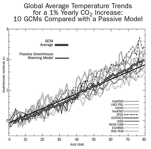
Figure 2a. Climate warming as projected by 10 state-of-the-art GCMs.17 The black and white line is the average of all 10 GCM projections, and the solid black line represents a passive greenhouse warming model as calculated by the author.
Figure 2a shows the temperature trends produced by 10 GCMs investigated in the “Coupled Model Intercomparison Project” (CMIP) at the Lawrence Livermore National Laboratory,17 showing what would happen if atmospheric CO2 were to increase at a steady 1% per year (about twice the current rate) for 80 years. The climate models excluded other “external forcings,” such as volcanic explosions, human-produced aerosols, and changes in solar intensity, but included internal feedbacks such as heat transfer between the oceans and the atmosphere, changes in snowfall, melting of ice caps, and so on. These GCMs are either identical with, or generally equivalent to, the GCMs used by the IPCC to predict the future temperatures of Earth climate in Figure 1 (SPM-5).
Along with the GCM projections, Figure 2a shows the trend from a very simple model, in which all that happens is passive greenhouse gas warming with no climate feedbacks at all. Nevertheless, for all its inherent simplicity, the passive warming line goes right through the middle of the GCM trend lines.
This result tells us that somehow the complex quintillion-watt feedbacks from the oceans, the atmosphere, the albedo, and the clouds all average out to approximately zero in the General Circulation Models. Apart from low intensity wiggles, the GCMs all predict little more than passive global warming.
All the calculations supporting the conclusions herein are presented in the Supporting Information (892KB PDF). Here’s the simplified greenhouse model in its entirety:
Global Warming=0.36x(33°C)x[(Total Forcing)÷(Base Forcing)]
Very complicated. The “33°C” is the baseline greenhouse temperature of Earth in Celsius, as defined by the year 1900.19 The “0.36” is the fraction of that greenhouse warming produced by CO2 plus the “enhanced water vapor feedback” that is said to accompany it.20 The enhancing idea is that as CO2 warms the atmosphere, more water vapor is produced. The extra water vapor in turn enhances the warming caused by CO2. The 0.36 is the fraction of greenhouse warming from water-vapor-enhanced CO2.21 All of this is detailed for critical inspection in SI Section 1.
The IPCC-approved equations10 were used to calculate the greenhouse gas forcings of CO2, methane, and nitrous oxide — the main additional greenhouse gases of today. That’s it. Nothing more complicated than algebra was involved.
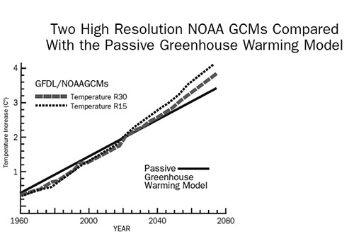
Figure 2b. The author’s passive warming model (solid black line) compared with the results from two high-resolution GCMs of the Geophysical Fluid Dynamics Laboratory (part of NOAA).18 All the projections in Figures 2a and 2b assume a yearly 1% compounded CO2 increase.
The GCM average line of Figure 2a (the black line with the white center) is the “ensemble average” of all ten GCM projections; that is, their sum divided by 10. Ensemble averages are typically accounted as more physically accurate than each individual GCM projection.22 By that criterion, the passive warming model is more physically accurate than any of the multi-million dollar CPU-burning GCMs, because it gets closer to the ensemble average than any of the 10 climate models (SI Section 2). Figure 2b shows a similar comparison with projections produced by two high-resolution GCMs of the Geophysical Fluid Dynamics Lab of NOAA,18 that included feedbacks from all known Earth climate processes. The simple model tracks their temperature projections more closely than many of the complex GCMs track one another.
Figure 2a shows that the physical model of Earth climate in GCMs says that as CO2 increases, Earth surface temperature does little else except passively respond in a linear way to greenhouse gas forcing. The same conclusion comes from looking at GCM control runs that project climate temperatures with constant atmospheric CO2. One of them is shown in Figure 1 — the “Year 2000” scenario. The line is nearly flat.
Since the satellite era especially, specific aspects of climate such as cloudiness or surface temperature have been monitored across the entire globe. GCM climate models can be tested by retrodiction — by making them reproduce the known past climate of Earth instead of the future climate. Physical error in GCMs can be quantified by comparing the retrodicted past with the real past.
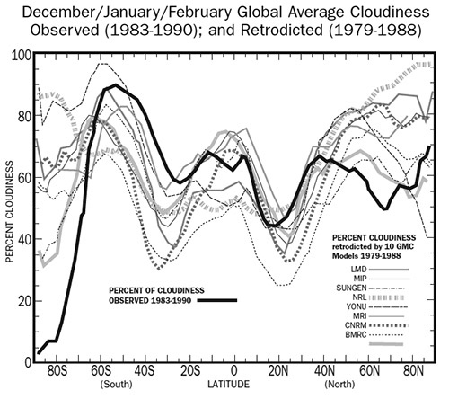
Figure 3. Heavy black line: observed cloudiness on Earth averaged over the years 1983–1990. Lighter and dotted lines: the average cloudiness on Earth over 1979–1988 as retrodicted by 10 revised General Circulation Models (GCMs). The GCMs identified by letter codes are detailed in Gates, et al.24
Figure 3 shows the December-January-February cloudiness observed by satellite on Earth, averaged over the years 1983–1990. It also shows global average cloudiness as retrodicted over the similar 1979–1988 period23 by 10 revised GCMs.24 The GCMs had been used in one attempt to reproduce the observed cloudiness, and were then revised and re-tested. This study was published in 1999, but the fidelity between GCM retrodictions and observed cloudiness has hardly improved in the past nine years.25
Looking at Figure 3, the GCMs do a pretty good job getting the general W-shape of Earth cloudiness, but there are significant misses by all the models at all latitudes including the tropics where clouds can have a large impact on climate.26 So, how wrong are the GCMs?
One approach to determining error is to integrate the total cloudiness retrodicted by each model and compare that to the total cloudiness actually observed (SI Section 3). Calculating error this way is a little simplistic because positive error in one latitude can be cancelled by negative error in another. This exercise produced a standard average cloudiness error of ±10.1%, which is about half the officially assessed GCM cloud error.24 So let’s call ±10.1% the minimal GCM cloud error.
The average energy impact of clouds on Earth climate is worth about -27.6 W/m2. 27 That means ±10.1% error produces a ±2.8 W/m2 uncertainty in GCM climate projections. This uncertainty equals about ±100 % of the current excess forcing produced by all the human-generated greenhouse gases presently in the atmosphere.10 Taking it into account will reflect a true, but incomplete, estimate of the physical reliability of a GCM temperature trend.
So, what happens when this ±2.8 W/m2 is propagated through the SRES temperature trends offered by the IPCC in Figure SPM-5 (Figure 1)? When calculating a year-by-year temperature projection, each new temperature plus its physical uncertainty gets fed into the calculation of the next year’s temperature plus its physical uncertainty. This sort of uncertainty accumulates each year because every predicted temperature includes its entire ± (physical uncertainty) range (SI Section 4).
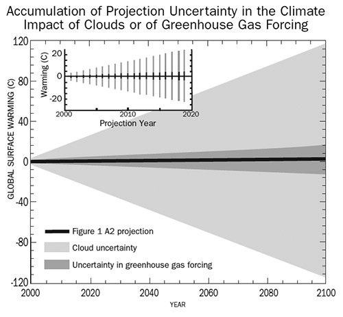
Figure 4. The Special Report on Emission Scenarios (SRES-SPM-5) A2 projection from Figure 1 showing the physical uncertainty of the projected temperature trend when including ±10.1% cloud error (light shading), or the uncertainty in greenhouse gas forcing (dark shading). Inset: A close-up view of the first 20 years of the A2 projection and the uncertainty limits.
Figure 4 shows the A2 SRES projection as it might have looked had the IPCC opted to show the minimal ±10.1 % cloud error as a measure of the physical accuracy of their GCM-scenarioed 21st century temperature trend. The result is a little embarrassing. The physical uncertainty accumulates rapidly and is so large at 100 years that accommodating it has almost flattened the steep SRES A2 projection of Figure 1. The ±4.4°C uncertainty at year 4 already exceeds the entire 3.7°C temperature increase at 100 years. By 50 years, the uncertainty in projected temperature is ±55°. At 100 years, the accumulated physical cloud uncertainty in temperature is ±111 degrees. Recall that this huge uncertainty stems from a minimal estimate of GCM physical cloud error.
In terms of the actual behavior of Earth climate, this uncertainty does not mean the GCMs are predicting that the climate may possibly be 100 degrees warmer or cooler by 2100. It means that the limits of resolution of the GCMs — their pixel size — is huge compared to what they are trying to project. In each new projection year of a century-scale calculation, the growing uncertainty in the climate impact of clouds alone makes the view of a GCM become progressively fuzzier.
It’s as though a stronger and stronger distorting lens was placed in front of your eyes every time you turned around. First the flowers disappear, then the people, then the cars, the houses, and finally the large skyscrapers. Everything fuzzes out leaving indistinct blobs, and even large-scale motions can’t be resolved. Claiming GCMs yield a reliable picture of future climate is like insisting that an indefinable blurry blob is really a house with a cat in the window.
The dark shading in Figure 4 shows the error due to uncertainties in greenhouse gas forcings themselves (~1% for CO2 ~10% for methane, ~5% for nitrous oxide),10 and how this small uncertainty accumulates during 100 years of climate projection. After a century, the uncertainty in predicted global average temperature is ±17 degrees just from accumulation of the smallish forcing error alone.
The difficulty is serious even over short times. The inset to Figure 4 shows that after only 20 years, the uncertainty from cloud error is ±22° and for forcing, it’s ±3°. The effect of the ~1% forcing uncertainty alone tells us that a 99% accurate GCM couldn’t discern a new Little Ice Age from a major tropical advance from even 20 years out. Not only are these physical uncertainties vastly larger than the IPCC allows in Figure SPM-5 (Figure 1), but the uncertainties the IPCC allows in Figure SPM-5 aren’t even physical.16
When both the cloud and the forcing uncertainties are allowed to accumulate together, after 5 years the A2 scenario includes a 0.34°C warmer Earth but a ±8.8°C uncertainty. At 10 years this becomes 0.44±15° C, and 0.6±27.7°C in 20 years. By 2100, the projection is 3.7±130°C. From clouds alone, all the IPCC projections have uncertainties that are very much larger than the projected greenhouse temperature increase. What is credible about a prediction that sports an uncertainty 20–40 times greater than itself? After only a few years, a GCM global temperature prediction is no more reliable than a random guess. That means the effect of greenhouse gases on Earth climate is unpredictable, and therefore undetectable. And therefore moot.
The rapid growth of uncertainty means that GCMs cannot discern an ice age from a hothouse from 5 years away, much less 100 years away. So far as GCMs are concerned, Earth may be a winter wonderland by 2100 or a tropical paradise. No one knows.
Direct tests of climate models tell the same tale. In 2002, Matthew Collins of the UK Hadley Centre used the HadCM3 GCM to generate an artificial climate, and then tested how the HadCM3 fared predicting the very same climate it had generated.28 It fared poorly, even though it was the perfect model. The problem was that tiny uncertainties in the inputs — the starting conditions — rapidly expanded and quickly drove the GCM into incoherence. Even with a perfect model, Collins reported that, “[I]t appears that annual mean global mean temperatures are potentially predictable 1 year in advance and that longer time averages are also marginally predictable 5 and 10 years in advance.” So with a perfect climate model and near-perfect inputs one might someday “potentially [predict]” and “marginally [predict],” but can not yet actually predict 1 year ahead. But with imperfect models, the IPCC predicts 100 years ahead.
Likewise, in a 2006 test of reliability, William Merryfield used 15 GCMs to predict future El Niño-Southern Oscillations (ENSO) in a greenhouse-warmed climate,29 and found that, “Under CO2 doubling, 8 of the 15 models exhibit ENSO amplitude changes that significantly (p<0.1) exceed centennial time scale variability within the respective control runs. However, in five of these models the amplitude decreases whereas in three it increases; hence there is no consensus as to the sign of change.” So of 15 GCMs, seven predicted no significant change, 5 predicted a weaker ENSO, and 3 predicted a stronger ENSO. This result is exactly equivalent to ‘don’t know.’ The 15 GCMs tested by Merryfield were the same ones used by the IPCC to produce its Fourth Assessment Report.
In light of all this, why is the IPCC so certain that human-produced CO2 is responsible for recent warming? How can the US National Academy of Sciences say, in a recent brochure, that, “ … Earth’s warming in recent decades has been caused primarily by human activities that have increased the amount of greenhouse gases in the atmosphere”?30 This brochure offers a very telling Figure 4 (SI Section 5), showing the inputs to 20th century global temperature from a GCM projection. Only when the effects of human greenhouse gases are included with normal temperature variation, we are told, does the GCM projected temperature trend match the observed temperature trend.
But their Figure 4 has another trait that is almost ubiquitous in GCM temperature projections. It shows no physical uncertainty limits. We are given a projected temperature trend that is implicitly represented as perfectly accurate. NAS Figure 4 would be more truthful if the National Academy presented it complete with ±100 degree uncertainty limits. Then it would be obvious that the correspondence between the observations and the projection was no more than accidental. Or else that the GCM was artificially adjusted to make it fit. It would also be obvious that it is meaningless to claim an explanatory fit is impossible without added CO2, when in fact an explanatory fit is impossible, period.
It is well-known among climatologists that large swaths of the physics in GCMs are not well understood.31 Where the uncertainty is significant GCMs have “parameters,” which are best judgments for how certain climate processes work. General Circulation Models have dozens of parameters and possibly a million variables,32 and all of them have some sort of error or uncertainty.
A proper assessment of their physical reliability would include propagating all the parameter uncertainties through the GCMs, and then reporting the total uncertainty.33 I have looked in vain for such a study. No one seems to ever have directly assessed the total physical reliability of a GCM by propagating the parameter uncertainties through it. In the usual physical sciences, an analysis like this is required practice. But not in GCM science, apparently, and so the same people who express alarm about future warming disregard their own profound ignorance.
So the bottom line is this: When it comes to future climate, no one knows what they’re talking about. No one. Not the IPCC nor its scientists, not the US National Academy of Sciences, not the NRDC or National Geographic, not the US Congressional House leadership, not me, not you, and certainly not Mr. Albert Gore. Earth’s climate is warming and no one knows exactly why. But there is no falsifiable scientific basis whatever to assert this warming is caused by human-produced greenhouse gases because current physical theory is too grossly inadequate to establish any cause at all.
Nevertheless, those who advocate extreme policies to reduce carbon dioxide emissions inevitably base their case on GCM projections, which somehow become real predictions in publicity releases. But even if these advocates admitted the uncertainty of their predictions, they might still invoke the Precautionary Principle and call for extreme reductions “just to be safe.” This principle says, “Where there are threats of serious or irreversible damage, lack of full scientific certainty shall not be used as a reason for postponing cost-effective measures to prevent environmental degradation.”34 That is, even if we don’t fully know that CO2 is dangerously warming Earth climate, we should curtail its emission anyway, just in case. However, if the present uncertainty limit in General Circulation Models is at least ±100 degrees per century, we are left in total ignorance about the temperature effect of increasing CO2. It’s not that we, “lack … full scientific certainty,” it’s that we lack any scientific certainty. We literally don’t know whether doubling atmospheric CO2 will have any discernible effect on climate at all.
If our knowledge of future climates is zero then for all we know either suppressing CO2 emissions or increasing them may make climate better, or worse, or just have a neutral effect. The alternatives are incommensurate but in our state of ignorance either choice equally has two chances in three of causing the least harm.35 Complete ignorance makes the Precautionary Principle completely useless. There are good reasons to reduce burning fossil fuels, but climate warming isn’t one of them.
Some may decide to believe anyway. “We can’t prove it,” they might say, “but the correlation of CO2 with temperature is there (they’re both rising, after all),36 and so the causality is there, too, even if we can’t prove it yet.” But correlation is not causation,37 and cause can’t be assigned by an insistent ignorance. The proper response to adamant certainty in the face of complete ignorance38 is rational skepticism. And aren’t we much better off accumulating resources to meet urgent needs than expending resources to service ignorant fears?
So, then, what about melting ice-sheets, rising sea levels, the extinction of polar bears, and more extreme weather events? What if unusually intense hurricane seasons really do cause widespread disaster? It is critical to keep a firm grip on reason and rationality, most especially when social invitations to frenzy are so pervasive. General Circulation Models are so terribly unreliable that there is no objectively falsifiable reason to suppose any of the current warming trend is due to human-produced CO2, or that this CO2 will detectably warm the climate at all. Therefore, even if extreme events do develop because of a warming climate, there is no scientifically valid reason to attribute the cause to human-produced CO2. In the chaos of Earth’s climate, there may be no discernible cause for warming.39 Many excellent scientists have explained all this in powerful works written to defuse the CO2 panic,40 but the choir sings seductively and few righteous believers seem willing to entertain disproofs.
Acknowledgments
The author thanks Prof. Carl Wunsch, Department of Earth, Atmospheric and Planetary Sciences, Massachusetts Institute of Technology, Prof. Paul Switzer, Department of Statistics, Stanford University, Prof. Ross McKitrick, Department of Economics, University of Guelph, Prof. Christopher Essex, Department of Applied Mathematics, University of Western Ontario, Prof. Sebastian Doniach, Departments of Physics and Applied Physics, Stanford University, Dr. Gerald L. Browning, Research Scientist (Emeritus), Cooperative Institute for Research in the Atmosphere (CIRA), Colorado State University, and Ms. Christine Adams, Redwood City, CA, for reviewing a prior version of this manuscript. The patience and consideration of Prof. McKitrick in performing all the Phillips-Perron tests in SI Section 4 is also very gratefully acknowledged. Any errors and all conclusions herein remain the sole responsibility of the author.
References
- McCarthy, J. 2005. “The Sustainability of Human Progress.” www.formal.stanford.edu/jmc/progress/ Last accessed on: 14 September 2007.
- Anon. 2006. “Consequences of Global Warming” National Resources Defense Council. www.nrdc.org/globalWarming/fcons.asp Last accessed on: 14 September 2007.
- Anon. 2007. “The Hard Facts of Global Warming.” The Sierra Club www.sierraclub.org/globalwarming/overview/overview4.asp Last accessed on: 14 September 2007.
- Anon. 2007. “Learning About the Science of Climate Change.” Greenpeace. www.greenpeace.org/international/campaigns/climatechange/science Last accessed on: 14 September 2007.
- Appenzeller, T. and D. R. Dimick. 2007. “Signs from Earth” National Geographic. http://magma.nationalgeographic.com/ngm/0409/feature1/ Last accessed on: 14 September 2007.
- Cicerone, R., E. J. Barron, R. E. Dickenson, I. Y. Fung, J. E. Hansen, et al. 2006. “Climate Change Science: An Analysis of Some Key Questions” The National Academy of Sciences, Washington, D.C. See also the 2006 report downloadable here: http://dels.nas.edu/basc/. Last accessed on: 14 September 2007.
- Pelosi, N. 2007. “We Will Work Together to Tackle Global Warming, One of Humanity’s Greatest Challenges.” www.speaker.gov/newsroom/speeches?id=0013 Last accessed on: 14 September 2007.
- Shermer. M. 2006. “The Flipping Point.” Scientific American 294, 28.
- Anon. Report FS-1999-06-025-GSFC: Earth’s Energy Balance, NASA: Goddard Space Flight Center Greenbelt, MD.
- Myhre, G., E. J. Highwood, K. P. Shine and F. Stordal. 1998. “New Estimates of Radiative Forcing Due to Well Mixed Greenhouse Gases.” Geophysical Research Letters 25, 2715–2718.
- Alley, R., T. Berntsen, N. L. Bindoff, Z. Chen, A. Chidthaisong, et al. “IPCC 2007: Summary for Policymakers.” In: Climate Change 2007: The Physical Science Basis. Cambridge University. http://ipcc-wg1.ucar.edu/wg1/wg1-report.html Last accessed on: 14 September, 2007. See under “WG1 Release”.
- The IPCC is careful to use “projection” rather than “prediction” to describe what GCMs produce. I.e., the words “predict” or “prediction” do not appear in the SPM of the 4AR. However, “projection” appears 20 times, “scenario” appears 50 times, and the peculiarly apt “storyline” is used 7 times. “Prediction” seems to be the default message for most readers, however.
- Soon, W., S. Baliunas, S. B. Idso, K. Y. Kondratyev, and E. S. Posmentier. 2001. “Modeling Climatic Effects of Anthropogenic Carbon Dioxide Emissions: Unknowns and Uncertainties” Climate Resear ch. 18, 259–275.
- Risbey, J. 2002. “Comment on Soon et al. (2001)” Climate Research 22, 185–186; W. Soon, S. Baliunas, S. B. Idso, K. Y. Kondratyev and E. S. Posmentier (2002). Reply to Risbey (2002) Climate Research 22, 187–188; D. J. Karoly, J. f. B. Mitchell, M. Allen, G. Hegerl, J. Marengo, et al. (2003) Comment on Soon et al. (2001) Climate Research 24, 91–92; W. Soon, S. Baliunas, S. B. Idso, K. Y. Kondratyev and E. S. Posmentier (2003). Reply to Karoly et al. (2003) Climate Research. 24, 93–94.
- One must go into Chapter 8 and especially Ch 8 Supplementary Material in the recently released IPCC 4AR to find GCM errors graphically displayed in W m-2. Figure S8.5, for example, shows that GCM errors in “mean shortwave radiation reflected to space” range across 25 W m-2. The errors in outgoing longwave radiation, Figure S8.7, are similarly large, and the ocean surface heat flux errors, Figure S8.14, minimally range across 10 W m-2. Such forthright displays do not appear in the SPM or in the Technical Summary; i.e., where public bodies are more likely to see them.
- The Legend of “The Physical Science Basis, Global Climate Projections” WGI analogous Figure 10.4 more cautiously advises that, “uncertainty across scenarios should not be interpreted from this figure (see Section 10.5.4.6 for uncertainty estimates).” However, in 10.5.4.6, it is not reassuring to read that, “[Uncertainty in future temperatures] results from an expert judgement of the multiple lines of evidence presented in Figure 10.29, and assumes that the models approximately capture the range of uncertainties in the carbon cycle.” And in WGI Chapter 8 Section 8.1.2.2: “What does the accuracy of a climate model’s simulation of past or contemporary climate say about the accuracy of its projections of climate change? This question is just beginning to be addressed … [T]he development of robust metrics is still at an early stage, [so] the model evaluations presented in this chapter are based primarily on experience and physical reasoning, as has been the norm in the past. (italics added)” That is, there is no validly calculated physical uncertainty limit available for any projection of future global climate.
- Covey, C., K. M. AchutaRao, U. Cubasch, P. Jones, S. J. Lambert, et al. 2003. “An overview of results from the Coupled Model Intercomparison Project” Global and Planetary Change, 37, 103–133; C. Covey, K. M. AchutaRao, S. J. Lambert and K. E. Taylor. “Intercomparison of Present and Future Climates Simulated by Coupled Ocean-Atmosphere GCMs” PCMDI Report No. 66 Lawrence Livermore National Laboratory 2001 http://www-pcmdi.llnl.gov/publications/pdf/report66/ Last accessed on: 14 September 2007.
- Dixon, K. R., T. L. Delworth, T. R. Knutson, M. J. Spelman and R. J. Stouffer. 2003. “A Comparison of Climate Change Simulations Produced by Two GFDL Coupled Climate Models.” Global and Planetary Change, 37, 81–102.
- Houghton, J. T., Y. Ding, D. J. Griggs, M. Noguer, P. J. van der Linden, et al. Climate Change 2001: The Scientific Basis. Chapter 1. The Climate System: An Overview. Section 1.2 Natural Climate Systems, Subsection 1.2.1 Natural Forcing of the Climate System: The Sun and the global energy balance. 2001 http://www.grida.no/climate/ipcc_tar/wg1/041.htm Last accessed on: 14 September 2007 “For the Earth to radiate 235 W m-2, it should radiate at an effective emission temperature of -19° C with typical wavelengths in the infrared part of the spectrum. This is 33° C lower than the average temperature of 14° C at the Earth’s surface.”
- Inamdar, A. K. and V. Ramanathan. 1998. “Tropical and Global Scale Interactions Among Water Vapor, Atmospheric Greenhouse Effect, and Surface Temperature.” Journal of Geophysical Research 103, 32,177–32,194.
- Manabe, S. and R. T. Wetherald. 1967. “Thermal Equilibrium of the Atmosphere with a given Distribution of Relative Humidity.” Journal of the Atmospheric Sciences 24, 241–259.
- Lambert, S. J. and G. J. Boer. 2001. “CMIP1 Evaluation and Intercomparison of Coupled Climate Models.” Climate Dynamics 17, 83–106.
- Rossow, W. B. and R. A. Schiffer. 1991. “ISCCP Cloud Data Products.” Bulletin of the American Meteorological Society 72, 2–20. Global average cloudiness does not change much from year-toyear. I.e., “Table 3 and Fig. 12 also illustrate how small the interannual variations of global mean values are. … All [the] complex regional variability appears to nearly cancel in global averages and produces slightly different seasonal cycles in different years.”
- Gates, W. L., J. S. Boyle, C. Covey, C. G. Dease, C. M. Doutriaux, et al. 1999. “An Overview of the Results of the Atmospheric Model Intercomparison Project.” (AMIP I) Bulletin of the American Meteorological Society 80, 29–55.
- AchutaRao, K., C. Covey, C. Doutriaux, M. Fiorino, P. Gleckler, et al. 2005. “Report UCRL-TR-202550. An Appraisal of Coupled Climate Model Simulations Lawrence Livermore National Laboratory.” See Figures 4.11 and 4.12. Especially compare Figure 4.11 with text Figure 3; M. H. Zhang, W. Y. Lin, S. A. Klein, J. T. Bacmeister, S. Bony, et al. 2005. “Comparing Clouds and Their Seasonal Variations in 10 Atmospheric General Circulation Models with Satellite Measurements.” Journal of Geophysical Research 110, D15S02 11–18.
- Hartmann, D. L. 2002. “Tropical Surprises.” Science, 295, 811–812.
- Hartmann, D. L., M. E. Ockert-Bell and M. L. Michelsen. 1992. “The Effect of Cloud Type on Earth’s Energy Balance: Global Analysis.” Journal of Climate 5, 1281–1304.
- Collins, M. 2002. “Climate Predictability on Interannual to Decadal Time Scales: The Initial Value Problem.” Climate Dynamics 19, 671–692.
- Merryfield, W. J. 2006. “Changes to ENSO under CO2 Doubling in a Multimodel Ensemble.” Journal of Climate 19, 4009–4027.
- Staudt, A., N. Huddleston and S. Rudenstein. 2006. “Understanding and Responding to Climate Change.” The National Academy of Sciences. http://dels.nas.edu/basc/ Last accessed on: 14 September 2007. The “low-res pdf” is a convenient download.
- Phillips, T. J., G. L. Potter, D. L. Williamson, R. T. Cederwall, J. S. Boyle, et al. 2004. “Evaluating Parameterizations in General Circulation Models.” Bulletin of the American Meteorological Society 85, 1903–1915.
- Allen M. R. and D. A. Stainforth. 2002. “Towards Objective Probabilistic Climate Forecasting.” Nature 419, 228; L. A. Smith. 2002. “What Might We Learn from Climate Forecasts?” Proceedings of the National Academy of Science, 99, 2487–2492.
- This is not the same as a sensitivity analysis in which the effects that variations in GCM parameters or inputs have on climate predictions are compared to observations. In contrast to this, propagating the errors through a GCM means the known or estimated errors and uncertainties in the parameters themselves are totaled up in a manner that quantitatively reflects their transmission through the mathematical structure of the physical theory expressed in the GCM. The total error would then represent the physical uncertainty in each and every prediction made by a GCM.
- Kriebel, D. J. Tickner, P. Epstein, J. Lemons, R. Levins, et al. 2001. “The Precautionary Principle in Environmental Science.” Environmental Health Perspectives 109, 871–876.
- Of course, reducing CO2 would likely stop the global greening that has been in progress since at least 1980. The Amazon rainforest alone accounted for 42% of the net global increase in vegetation: R. R. Nemani, C. D. Keeling, H. Hashimoto, W. M. Jolly, S. C. Piper, et al. 2003. “Climate-Driven Increases in Global Terrestrial Net Primary Production from 1982 to 1999.” Science 300, 1560–1563; S. Piao, P. Friedlingstein, C. P., L. Zhou and A. Chen. 2006. “Effect of Climate and CO2 Changes on the Greening of the Northern Hemisphere Over the Past Two Decades.” Geophysical Research Letters 33, L23402 23401–23406.
- Rising CO2 correlates strongly (r2=0.71) with the greening of the Sahel since 1980, too. SI Section 6.
- Aldrich, J. 1995. “Correlations Genuine and Spurious in Pearson and Yule.” Statistical Science 10, 364–376. In 1926 G. Udny Yule famously reported a 0.95 correlation between mortality rates and Church of England marriages.
- On the other hand, the history of Earth includes atmospheric CO2 lagging both glaciations and deglaciations, and large rapid spontaneous jumps in global temperatures without any important changes in atmospheric CO2 and without tipping Earth off into runaway catastrophes. See references for the Dansgaard-Oeschger events, for example: Adams, J. M. Maslin and E. Thomas. 1999. “Sudden Climate Transitions During the Quaternary.” Progress in Physical Geography 23, 1–36; G. G. Bianchi and I. N. McCave. 1999. “Holocene Periodicity in North Atlantic Climate and Deep Ocean Flow South of Iceland.” Nature 397, 515–517; M. McCaffrey, D. Anderson, B. Bauer, M. Eakin, E. Gille, et al. 2003. “Variability During the Last Ice Age: Dansgaard-Oeschger Events.” NOAA Satellites and Information. http://www.ncdc.noaa.gov/paleo/abrupt/data_glacial2.html Last accessed on: 14 September 2007; L. C. Gerhard. 2004. “Climate change: Conflict of Observational Science, Theory, and Politics.” AAPC Bulletin 88, 1211–1220.
- J. M. Mitchell Jr. 1976 “An overview of climatic variability and its causal mechanisms” Quaternary Research 6, 481–493. Shao, Y. 2002. C. Wunsch 2003 “The spectral description of climate change including the 100 ky energy” Climate Dynamics 20, 253–263. “Chaos of a Simple Coupled System Generated by Interaction and External Forcing.” Meteorology and Atmospheric Physics 81, 191–205; J. A. Rial 2004. “Abrupt Climate Change: Chaos and Order at Orbital and Millennial Scales.” Global and Planetary Change 41, 95–109.
- Lindzen, R. S. 1997. “Can Increasing Carbon Dioxide Cause Climate Change?” Proceedings of the National Academy of Science, 94, 8335–8342; W. Soon, S. L. Baliunas, A. B. Robinson and Z. W. Robinson. 1999. “Environmental Effects of Increased Carbon Dioxide.” Climate Research 13, 149–164; C. R. de Freitas. 2002. “Are Observed Changes in the Concentration of Carbon Dioxide in the Atmosphere Really Dangerous?” Bulletin of Canadian Petroleum Geology 50, 297–327; C. Essex and R. McKitrick. 2003. “Taken by Storm: The Troubled Science, Policy, and Politics of Global Warming” Key Porter Books: Toronto; W. Kininmonth. 2003. “Climate Change: A Natural Hazard.” Energy & Environment 14, 215–232; M. Leroux. 2005. “Global Warming — Myth or Reality?: The Erring Ways of Climatology”. Springer: Berlin; R. S. Lindzen. 2006. “Is There a Basis for Global Warming Alarm?” In Global Warming: Looking Beyond Kyoto Ed. Yale University: New Haven, in press. The full text is available at: http://www.ycsg.yale.edu/climate/forms/LindzenYaleMtg.pdf Last accessed: 14 September 2007.
This article can be found in

volume 14 number 1
A Climate of Belief
How We Know Global Warming is Real: The Science Behind Human-induced Climate Change; How to solve the global warming problem by 2020…
BROWSE this issue >
ORDER this issue >
This article was published on February 23, 2011.